BOP Challenge 2019

1. Introduction

This page defines the 2019 edition of the BOP Challenge on pose estimation of specific rigid objects. As the evaluation methodology stayed intact in the succeeding 2020 and 2022 editions, the leaderboard is shared by all three editions and the submission form for this leaderboard stays open to allow comparison with upcoming methods.

2. Important dates

• Submission deadline: October 21, 2019 (11:59PM PST). The submission form stays open even after the deadline.
• Presentation of awards: October 28, 2019 (at the R6D workshop at ICCV 2019).

3. Task definition

The challenge is on the task of 6D localization of a varying number of instances of a varying number of objects in a single RGB-D image (the ViVo task).

The ViVo task is referred to as the 6D localization problem in [2]. In the BOP paper [1], methods were evaluated on a different task – 6D localization of a single instance of a single object (the SiSo task), which was chosen because it allowed to evaluate all relevant methods out of the box. Since then, the state of the art has advanced and we have moved to the more challenging ViVo task.

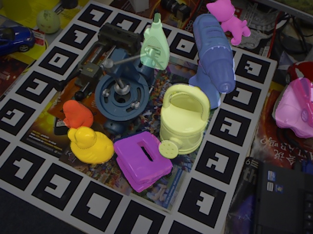
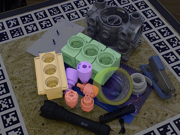
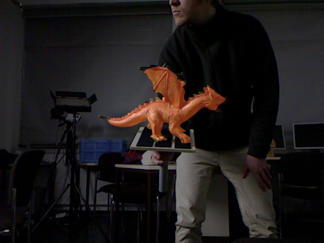
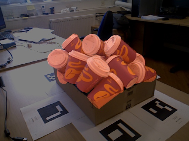
4. Datasets

Multiple datasets are used for the evaluation. Each dataset is provided in the BOP format and includes 3D object models and training and test RGB-D images annotated with ground-truth 6D object poses. Some datasets (HB, ITODD) include also validation images – in this case, the ground-truth poses are publicly available only for the validation images, not for the test images. The object models were created manually or using KinectFusion-like systems for 3D surface reconstruction [6]. The training images were either captured by an RGB-D/Gray-D sensor or obtained by rendering of the object models. The test images were captured in scenes with graded complexity, often with clutter and occlusion.

For training, a method can use the provided object models and training images. It can also render extra training images using the models. Not a single pixel of test images may be used for training, nor the individual ground-truth poses or object masks provided for the test images. The range of all ground-truth poses in the test images, which is provided in file dataset_params.py in the BOP toolkit (items depth_range, azimuth_range, and elev_range), is the only information about the test set that can be used for training.

4.1 List of datasets

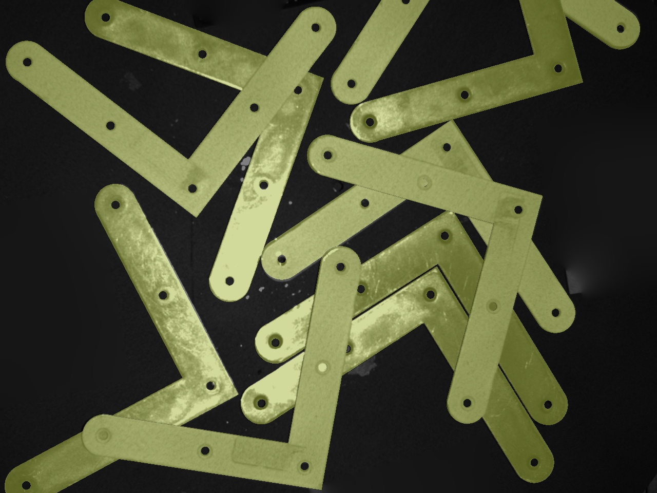
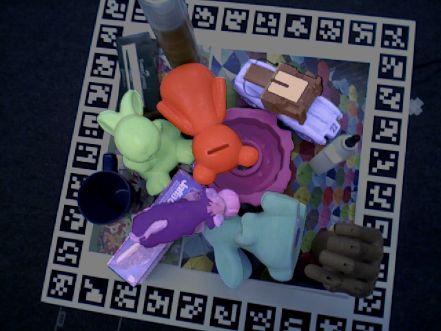
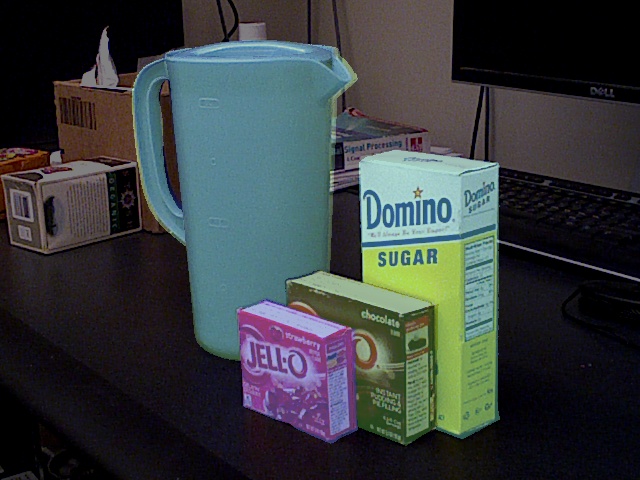
Core datasets: LM-O, T-LESS, TUD-L, IC-BIN, ITODD, HB, YCB-V. A method needs to be evaluated on these seven datasets to be considered for the main awards.
Other datasets: LM, RU-APC, IC-MI, TYO-L.

Only subsets of the original datasets are used to speed up the evaluation. The subsets are defined in files test_targets_bop19.json provided with the datasets.

5. Awards

• The Overall Best Method – The top-performing method on the seven core datasets.
• The Best RGB-Only Method – The top-performing RGB-only method on the seven core datasets.
• The Best Fast Method – The top-performing method on the seven core datasets with the average running time per image below 1s.
• The Best Open-Source Method – The top-performing method on the seven core datasets whose source code is publicly available.
• The Best Method on Dataset D – The top-performing method on each of the available datasets.

See conditions which a method needs to fulfill in order to qualify for the awards.

The BOP Challenge 2019 awards were presented at the 5th Workshop on Recovering 6D Object Pose (ICCV 2019, Seoul).

6. How to participate

To have your method evaluated, run it on the ViVo task and submit the results in the format described below to the evaluation system (the evaluation script used in the system is publicly available). Note that each method has to use an identical set of hyper-parameters across all objects and datasets.

The list of object instances for which the pose is to be estimated can be found in files test_targets_bop19.json provided with the datasets. For each object instance in the list, at least $10\%$ of the object surface is visible in the image [1].

6.1 Format of results

Results for all test images from one dataset are saved in one CSV file named METHOD_DATASET-test.csv, with one pose estimate per line in the following format:

scene_id,im_id,obj_id,score,R,t,time

• scene_id, im_id, and obj_id is the ID of scene, image and object respectively.
• score is a confidence of the estimate (the range of confidence values is not restricted).
• R is a 3x3 rotation matrix whose elements are saved row-wise and separated by a white space (i.e. r11 r12 r13 r21 r22 r23 r31 r32 r33, where rij is an element from the i-th row and the j-th column of the matrix).
• t is a 3x1 translation vector (in mm) whose elements are separated by a white space (i.e. t1 t2 t3).
• time is the time the method took to estimate poses for all objects in image im_id from scene scene_id. All estimates with the same scene_id and im_id must have the same value of time. Report the wall time from the point right after the raw data (the image, 3D object models etc.) is loaded to the point when the final pose estimates are available (a single real number in seconds, -1 if not available).

$\mathbf{C} = \mathbf{K} [\mathbf{R} \, \mathbf{t}]$ is the camera matrix which transforms a 3D point in the model coordinate system, $\mathbf{x}_m = [x, y, z, 1]'$, to a 2D point in the image coordinate system, $\mathbf{x}_i = [u, v, 1]'$: $s\mathbf{x_i} = \mathbf{C} \mathbf{x}_m$. The camera coordinate system is defined as in OpenCV with the camera looking along the $Z$ axis. The intrinsic matrix $\mathbf{K}$ is provided with the test images – note it may be different for each image.

Example results can be found here.

6.2 Terms & conditions

1. To be considered for the awards and for inclusion in a publication about the challenge, the authors need to provide documentation of the method (including specifications of the used computer) through the online submission form.
2. The winners need to present their methods at the awards reception.
3. After the submitted results are evaluated (by the online evaluation system), the authors can decide whether to make the scores visible to the public.

7. Evaluation methodology

7.1 Pose-error functions

The error of an estimated pose $\hat{\textbf{P}}$ w.r.t. the ground-truth pose $\bar{\textbf{P}}$ of an object model $M$ is measured by three pose-error functions defined below. Their implementation is available in the BOP toolkit.

Visible Surface Discrepancy (VSD) [1,2]:

where $\hat{D}$ and $\bar{D}$ are distance maps obtained by rendering the object model $M$ in the estimated pose $\hat{\textbf{P}}$ and the ground-truth pose $\bar{\textbf{P}}$ respectively. The distance maps are compared with the distance map $D_I$ of the test image $I$ to obtain the visibility masks $\hat{V}$ and $\bar{V}$, i.e. the sets of pixels where the model $M$ is visible in image $I$. Compared to [1,2], the estimation of visibility masks has been modified – at pixels with no depth measurements, an object is now considered visible (it was considered not visible in [1,2]). This modification allows evaluating poses of glossy objects from the ITODD dataset whose surface is not always captured by the depth sensors. $\tau$ is a misalignment tolerance.

VSD treats indistinguishable poses as equivalent by considering only the visible object part. See Section 2.2 of [1] and FAQ for details.

Maximum Symmetry-Aware Surface Distance (MSSD) [3]:

where $S_M$ is a set of global symmetry transformations and $V_M$ is a set of mesh vertices of object model $M$ (see Section 5.2).

The maximum distance is relevant for robotic manipulation, where the maximum surface deviation strongly indicates the chance of a successful grasp. Moreover, compared to the average distance used in ADD/ADI [2, 5] which tends to be dominated by higher-frequency surface parts, the maximum distance is less dependent on the sampling of mesh vertices.

Maximum Symmetry-Aware Projection Distance (MSPD):

where $\text{proj}$ is the 2D projection operation (the result is in pixels) and the meaning of the other symbols is as in MSSD.

Compared to the 2D projection [4], MSPD considers global object symmetries and replaces the average by the maximum distance to increase robustness against the sampling of mesh vertices. Since MSPD does not evaluate the alignment along the optical axis (Z axis) and measures only the perceivable discrepancy, it is relevant for augmented reality applications and suitable for evaluating RGB-only methods.

7.2 Identifying global object symmetries

The set of global symmetry transformations of an object (used in MSSD and MSPD) is identified in two steps. Firstly, we obtain a set of candidate symmetry transformations as $S'_M = \{\textbf{S}: h(V_M, \textbf{S}V_M) < \varepsilon \}$, where $h$ is the Hausdorff distance calculated between vertices $V_M$ of object model $M$ in the canonical and transformed locations. The allowed deviation is bounded by $\varepsilon = \text{max}(15\,mm, 0.1d)$, where $d$ is the diameter of model $M$ (the largest distance between any pair of model vertices) and the truncation at $15\,mm$ avoids breaking the symmetries by too small details. Secondly, we identify the final set of symmetry transformations $S_M$ as a subset of $S'_M$ which consists of those symmetry transformations that cannot be resolved by the model texture (decided subjectively by the organizers of the challenge).

Set $S_M$ covers both discrete and continuous global rotational symmetries. The continuous rotational symmetries are discretized such as the vertex which is the furthest from the axis of symmetry travels not more than $1\%$ of the object diameter between two consecutive rotations. The symmetry transformations are stored in files models_info.json provided with the datasets.

7.3 Performance score

An estimated pose is considered correct w.r.t. pose-error function $e$ if $e < \theta_e$, where $e \in \{e_{\text{VSD}}, e_{\text{MSSD}}, e_{\text{MSPD}}\}$ and $\theta_e$ is the threshold of correctness. The fraction of annotated object instances, for which a correct pose is estimated, is referred to as recall. The Average Recall w.r.t. function $e$, denoted as $\text{AR}_e$, is defined as the average of the recall rates calculated for multiple settings of threshold $\theta_e$, and also for multiple settings of the misalignment tolerance $\tau$ in the case of $e_{\text{VSD}}$.

• $\text{AR}_\text{VSD}$ is the average of recall rates calculated for the misalignment tolerance $\tau$ ranging from $5\%$ to $50\%$ of the object diameter with a step of $5\%$, and the threshold of correctness $\theta_{\text{VSD}}$ ranging from $0.05$ to $0.5$ with a step of $0.05$.
• $\text{AR}_\text{MSSD}$ is the average of recall rates calculated for $\theta_{\text{MSSD}}$ ranging from $5\%$ to $50\%$ of the object diameter with a step of $5\%$.
• $\text{AR}_\text{MSPD}$ is the average of recall rates calculated for $\theta_{\text{MSPD}}$ ranging from $5r$ to $50r$ with a step of $5r$, where $r = w/640$ and $w$ is the width of the image in pixels.

The performance of a method on a dataset is measured by the Average Recall: $\text{AR} = (\text{AR}_{\text{VSD}} + \text{AR}_{\text{MSSD}} + \text{AR}_{\text{MSPD}}) / 3$. The overall performance on the core datasets is measured by $\text{AR}_{\text{Core}}$ defined as the average of the per-dataset $\text{AR}$ scores. In this way, each dataset is treated as a separate sub-challenge which avoids $\text{AR}_{\text{Core}}$ being dominated by larger datasets.

8. FAQ

8.1 Why synthetic training images?

While 3D object models are often available or can be generated at a low cost using KinectFusion-like systems for 3D surface reconstruction [6], capturing and annotating real training images requires a significant effort. The challenge is therefore focused primarily on the more practical scenario where only the object models, which can be used to render synthetic training images, are available at training time.

8.2 6D localization vs. 6D detection

Prior information about the object presence in the input image distinguishes two 6D object pose estimation tasks: 6D localization, where the identifiers of present object instances are provided for each image, and 6D detection, where no prior information is provided [2].

The aspect which is evaluated on the 6D detection but not on the 6D localization task is the capability of the method to calibrate the predicted confidence scores across all object classes. For example, a score of $0.5$ for a cat should represent the same level of confidence as a score of $0.5$ for a duck. This calibration is important for achieving good performance w.r.t. the precision/recall curve which is typically used for evaluating detection. The 6D localization task still requires the method to sort the hypotheses, although only within the same object class – the method needs to output the top N pose estimates for an object class which are evaluated against N ground-truth poses of that class.

There are two reasons why the methods are evaluated on the 6D localization task in BOP:

1. 6D detection has computationally expensive evaluation as many more hypotheses need to be evaluated to calculate the precision/recall curve. Calculating the 6D pose errors is more expensive than e.g. calculating the intersection over union of 2D bounding boxes (used to evaluate 2D object detection).
2. The scores on the simpler 6D localization task are far from being saturated.

8.3 Discussion on the pose-error functions

Evaluating 6D object pose estimates is not straightforward. Only a fraction of an object’s surface may be visible in an image due to self-occlusion and occlusion by other objects. The visible part of the object may have multiple fits to the object’s 3D model. As a consequence, there may be (infinitely) many 6D poses consistent with the image. It is often difficult to explicitly enumerate all consistent poses.

The most widely used pose-error functions have been ADD/ADI [2,5], where the error is calculated as the average distance from vertices of the object model in the ground-truth pose to vertices of the model in the estimated pose. The distance is measured between corresponding vertices if all views of the object are distinguishable (ADD). Otherwise, for objects with indistinguishable views, the distance is measured between a given vertex and its nearest neighbor in 3D space, which may not necessarily be the corresponding vertex (ADI). ADI can yield un-intuitively low errors even for poses that are distinguishable. Objects evaluated with ADI therefore tend to yield low pose errors although the estimated poses might not be visually well aligned. Another limitation of ADD/ADI comes from a high dependence on the geometry of the object model and the sampling density of its surface – the average distance is dominated by higher-frequency surface parts, such as the thread of a fuse. The maximum distance used in MSSD and MSPD is less dependent on the surface sampling density.

MSSD and MSPD handle pose ambiguities due to global object symmetries. MSSD is suitable for robotic grasping and MSPD for augmented reality applications. However, because both are calculated over the entire model surface, misalignments of invisible parts are penalized. This may not be desirable for applications such as robotic manipulation with suction cups where only the alignment of the visible part is relevant. VSD is calculated only over the visible object part. It evaluates the alignment of the object shape but not of its color – this is because most of the object models currently included in BOP have baked shadows and reflections in their textures, which makes it difficult to robustly evaluate color alignment. As each of VSD, MSSD and MSPD is relevant for a different target application, we use all three for the evaluation in BOP.

9. Organizers

Tomáš Hodaň, Czech Technical University in Prague
Martin Sundermeyer, DLR German Aerospace Center
Eric Brachmann, Heidelberg University
Bertram Drost, MVTec
Frank Michel, Technical University Dresden
Jiří Matas, Czech Technical University in Prague
Carsten Rother, Heidelberg University

References

[1] Hodaň, Michel et al.: BOP: Benchmark for 6D Object Pose Estimation, ECCV 2018.

[2] Hodaň et al.: On Evaluation of 6D Object Pose Estimation, ECCVW 2016.

[3] Drost et al.: Introducing MVTec ITODD - A Dataset for 3D Object Recognition in Industry, ICCVW 2017.

[4] Brachmann et al.: Uncertainty-Driven 6D Pose Estimation of Objects and Scenes from a Single RGB Image, CVPR 2016.

[5] Hinterstoisser et al.: Model based training, detection and pose estimation of texture-less 3d objects in heavily cluttered scenes, ACCV 2012.

[6] Newcombe et al.: KinectFusion: Real-time dense surface mapping and tracking, ISMAR 2011.